GUI¶

Trac^x also features a graphical user interface (GUI). The purpose of the GUI is to guide the user quickly through the necessary steps to conduct a tracking experiment, view the results and provide an overall more intuitive interface for users who have limited coding experience or who just want to quickly test the Trac^x algorithm without a lot of prior time investment. In principle, the GUI writes and executes a basic Trac^x script for the user in the background. However, if the goal is to create a pipeline for many datasets with custom analysis steps and large amounts of data, the user is advised to resort to the coding interface nonetheless, as the GUI was not designed with this purpose in mind.

A quick introduction for new users who jumped directly to the GUI¶

Please note, that just like for the code interface, the input data needs to fulfill certain requirements. The GUI contains some functionalities to transform your data to the correct format.

General input data requirements:

A set of brightfield or fluorescence microscopy images in the form of TIF files, one file per timepoint, position, channel, etc. These images will be used for the Trac^x fingerprints.
A corresponding set of segmentation masks (segmented cells or nuclei). The segmentation masks need to be generated by third-party software (e.g. CellX or Cellpose or similar), as Trac^x does not include a segmentation functionality. Labeled masks are preferred over binary masks. These files should also be provided as TIF files and have the same image dimensions as the raw images.
Optional: Any number of additional fluorescence channels that will then be quantified by the algorithm, provided in the same file format and image dimensions.

File names:

Ideally, the file names take the format ChannelName_positionXXYYZZZ_timeTTTT.tif, e.g. Brightfield_position0101000_time0001.tif. Position refers to the x and y component of the well position and to the z-plane; it can be set to 0101000 as a default, if this does not apply to your experiment. The GUI contains a name parser interface that can be used to transform your original file names to the Trac^x format using MATLAB? regular expressions, if they do not yet conform to this format (see extended guide below).

Specific requirements for 3D-data (3D + time):

The file format should be in the form of one z-stack per timepoint and channel, as a multi-page TIF file containing the z-planes. If all z-planes are provided as separate files, or all planes and timepoints are provided as one single frame, these can be transformed in the GUI. However, the channels need to be separate.

Note

The Trac^x GUI requires MATLAB R2020a or newer.

Main window¶

The main window of Trac^x.

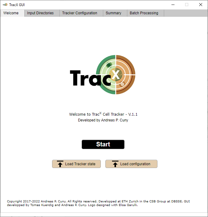
To start a new project from scratch click on Start. Otherwise a project can be loaded from a project file (.xml) or from a previous Trac^x state (.mat).

Input directories tab¶

To initialize a new project:

Enter the path to the segmentation results or click on Search to open a dialog to help you selecting the segmentation results folder.
Select the folder containing the raw images.
(optional) If you imaged additional channels, you can add their file prefixes as well, separated by a comma (i.e GFP, YFP). All additional channels need to be added if they need to be quantified by Prepare Segmentation Data. Otherwise only the channel required for the asymmetric lineage reconstruction needs to be entered (i.e. budneck marker).
Adjust the filter to identify the mask and image files properly. If your mask file is i.e termed mask_time001.mat set the filter to mask*.mat. Same for the image i.e. BF_position010100_time0001.tif the filter should be set to BF*.tif
Hit Evaluate. If everything is ok, the Continue button will be enabled. If not, you find information in the text field on the left about what went wrong and what to do in order to resolve the problem.

One major cause of problems could be that your segmentation data is not in the proper format. This is the case if your input are labeled segmentation masks. To convert them into the proper format hit the Prepare Segmentation Data button which initiates the conversion and then hit Evalute again. Another cause especially for 3D data could be that each timepoint and each plane is saved as individual tif file and not as stack. To convert hit Stacking single planes.

Note

In general, we need the same amount of segmentation data as image data files. Additionally the segmentation mask and image file dimensions need to be identical.

Troubleshooting:

If you need to ‘Prepare Segmentation Data’ from your own or any other segmentation algorithm such as showcased by the demo data (Demo data , datayeastscerevisiaeGenericSegmentation example) and including quantification from additional fluorescent channels it must be entered as follows:

Add the path to the segmentation files (for demo data i.e. datayeastscerevisiaeGenericSegmentation)
Add the path to the segmentation images (for demo data i.e datayeastscerevisiaeRawImages)
Add (optional) channels to be quantified (for demo data i.e ‘mKOk’ ‘mKate’) other wise the field for Additional Channels must remain empty.
Adjust the regular expression filters to identify the image file names and the segmentation file names (for demo data i.e. “BFdivide_*.tif” and “mask*.tif”)
Hit Evalute and check the log and then Prepare Segmentation Data and you should read in the log the following:

INFO: Started CellXMask extractor with following parameters:
          flatFieldFileNames: {}
                    fluoTags: {'mKOk'  'mKate'}
          imageFileNameRegex: 'BFdivide_*.tif'
                   imagePath: 'E:\tracx_demo_data\scripts\..\data\yeast\scerevisiae\RawImages'
                  pxPerPlane: 0
   segmentationFileNameRegex: 'mask*.tif'
            segmentationPath: 'E:\tracx_demo_data\scripts\..\data\yeast\scerevisiae\GenericSegmentation'

If you got an error _invalid fluoTags_ then please check that you entered the Additional Channels as described above. If you received an error for _ERROR: Index exceeds the number of array elements (0)._ please check that you entered the regular expressions properly for Mask file filter and Image file filter to identify the image and/or segmentation files and check that the mask file names follow our naming convention (ChannelName_positionXXYYZZZ_timeTTTT.tif, e.g. Brightfield_position0101000_time0001.tif).

At the bottom there are additionally two windows:

Log: Shows the console output of Trac^x
Command Window: Lets you interact with Trac^x as if you would work with it in an open Matlab session. However only methods of Trac^x can be evaluated. This is helpful to inspect a current state of Trac^x or display a certain image frame with certain properties such as i.e.Tracker.imageVisualization.plotAnnotatedControlImageFrame(10, ‘cell_area’) which would show an image of frame 10 with each cell labeled by its area.

Tracker configuration tab¶

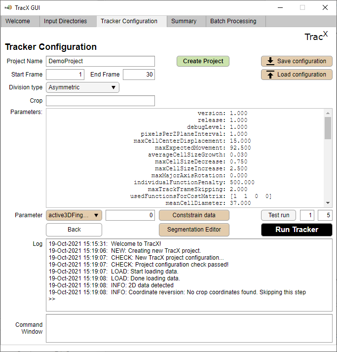
Trac^x configuration

Set a project name
Set from where to where to track the data (image frames).
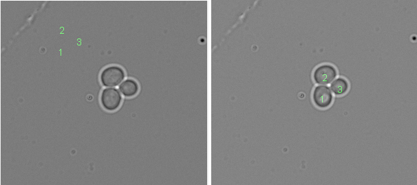
Define what is the cell division type. For asymmetrically dividing cells such as the yeast S.cerevisiae choose Asymmetrical. For symmetrically dividing cells such as bacteria or rod shaped yeast S.pombe choose Symmetrical. For convex shaped cells such as cell nuceli, mESC, HELA etc choose Mammalian.
(optional) Define an image crop. If you used CellX to segment your dataset and used a cropped region you need to enter the crop coordinates found in the CellX Parameter file to match the segmentation results with the full image size. The coordinates should be entered as four numbers separated by a comma i.e. 73, 71, 179, 174. This parameter should only be used if CellX has been used for segmentation! If you want to crop the image, use the Constrain data editor. For more information, see the section Constrain data.
Set the parameters. For most datasets the default parameters are just fine. For detailed description of each parameter please see Description of the tracker parameters. To set a specific parameter choose it from the drop down value which will then display its current value on the right and let you modify its value. Hit Enter to apply the change.
Hit Create Project to create a the Trac^x. At this point you can also save the project by hitting the Save configuration button which will save all the project information you just entered in an .xml file.
Run Trac^x by clicking on Run Tracker.

Optionally you can also load an existing Trac^x configuration by clicking on Load configuration.

If you want to track only a specific subset of cells on your images or you know you have quite some segmentation artefacts you can constrain your input data by clicking Constrain data prior to running Trac^x. For more information see below in the section Constrain data.

If you know that on some frames the segmentation was particularly bad or you want to fix certain mistakes or add new cells you can do this manually by clicking on the Segmentation editor. For more information see below in the section Segmentation editor.

Below the effect of point 4 from above is shown if the CellX segmentation is used that was run with an image crop. If not corrected, the cell coordinates do not map properly to the images.

Summary tab¶

Tracking Summary

Provides you with a quick overview and statistics of the tracking results as well as a visual for the distribution of track lenghts over time. Distribution of track lengths shows a histogram of the lengths of the tracks found throughout the timeseries. Distribution of tracks over time shows a column plot which represents for each frame in the timeseries: the total number of tracks in that frame ‘All’, the number of newly started tracks in that frame ‘New’ and the number of tracks that end in that frame ‘End’.

If all looks good you can hit Save Tracker state if you wish to keep the current state or work with the tracked data at a later time. Optionally you can also hit Save control images to export some control images and tracked segmentation masks.
To visualize the results of any segmentation property you can open the View results which also allows to export animated movies.
If you like to continue work in the Matlab IDE you can also export a Matlab scribt with Generate Script. Optionally you can now also reconstruct the cell lineage. Make sure that the correct cell division type is selected.
If the tracking results do not look how you expected you can either go back to the Tracker Configuration and try different parameters or fix tracking or lineage reconstruction errors manually by clicking onto Troubleshooting. This opens a new window for manual corrections. For details see below in the Manual corrections section.
If you started Trac^x from the Matalb IDE you can also export the Trac^x object into Matlabs workspace. Tick the Export Tracker Object to worksspace and select a handle name for it. It defaults to Tracker, before clicking Exit button.

At this point tracking is done and you can start with the data analysis.

Batch processing tab¶

Batch Processing

If you have many experiments to track, i.e a multi well plate or multi position experiment you can create Trac^x scripts or Trac^x project configurations for each of the position, save them and then load them here for batch processing. Trac^x will then run them all for you. To select the files click on Add files and then click on Run Batch.

To check on the progress (refresh the log window) you can click on the Check status button.

File converter¶

The file converter of Trac^x lets you import segmentation results from any segmentation algorithm of your choice. It will convert the data into a standardized format used internally by Trac^x. It also allows to rename images as well as destack multi-page tiffs for frame to frame processing.

File name converter tab¶

File name converter The file name converter allows you to convert your custom image / file names as saved by your acquisition software into a format that Trac^x understands. It follows the filename convention of YouScope (an opensource microscope aquisition software based on Micro Manager). The format is the following: ChannelName_WellPositionZPosition_Time.tif

With the help of regular expressions (examples are present for help in the fields directly) you can detect the identifiers (i.e Channel) from your filenames and then rename them by custom identifiers or keep how they were saved.

At the bottom there is a preview of the original file names and how they will be termed after convertion. If you have additional fluorescence channels which are encoded by numbers in your original filenames ie. *c1*, *c4*etc you can rename them by entering a comma-separated list i.e 1, PhC, 4, GFP.

When you click on Run conversion the image names will be converted while the raw image files will be kept in a subfolder as backup.

Stacking single planes tab¶

Stacking single planes

If you have a 3D dataset present as all single-page tiff files with the z and time position encoded in the name you can ajust the regular expression to detect the z position in your names and create a multi-page stacked tiff file. The preview indicates how the sucessfull stacking would look like before clicking the Run stacking button. The expected output is a series of z stacks (one per timepoint) per tiff file.

If needed, the stacking can be reverted by clicking Revert previous stacking

Destacking timepoints tab¶

Destacking timepoints

If your 3D data is all in one file (i.e all timepoints and all z planes) you can use this function to convert the data into a seris of timepoints. The required inputs are the number of expected timepoints and the number of z planes as well as the order in which they are stored in the multi page tiff file (i.e if first all z-planes for the first timepoint or if for the first z-plane all timepoints are stored)

Click on Destack (optional) to destack the multi-page tiff file. You can use the functions for segmentation masks or images of your experiment. The expected output is a series of z stacks (one per timepoint) per tiff file.

If needed, the destacking can be reverted by clicking Revert previous destacking

Segmentation editor¶

The segmentation editor of Trac^x lets you modify imperfect segmentations manually. You can delete, add or modify any segmentation object and requantify the changes. At any given time you can rollback the changes if needed.

To draw a new segmentation hit Add new segmentation and then click onto the image to trace your cells and entering vertices. Trac^x tries to predict the cell membrane based on gradients to help you segment the cell automatically. In some cases this does not work you you need to make smaller distances and add more vertices to get the outline correct. If you misplaced a vertex just right click with the mouse on the outline which opens a small window and lets you delete this vertex again.
To delete a bad segmentation click onto it in the Working area and then hit Delete selected. If you did some mistakes you can always revert to the original segmentation at any point. Please note you will loose all modifications on that frame!
Save changes on current frame saves all the manual changes you made for this frame and lets you continue with a different frame. Also if you change to a different frame without saving, it will turn to a red background and ask you to either discard all the changes on that frame or save them (see image below).
Click Apply & Close once you are happy with all edits. This will finally apply all your changes and re quantify your images for all the frames you edited manually. This process is done in parallel but still might take some time. Once done you will return to Trac^x main window.

In the toolbar top left you can activate zoom in, zoom out, drag as well as switch the Segmentation Preview area on the right between labeled masks or a transparent binary preview showing the pixels that would be segmented by the mask from the raw image (see image below).

At the bottom you find a slider to navigate trough your image set. With the buttons you can jump to the very first or very last frame or jump in steps of 10 frames.

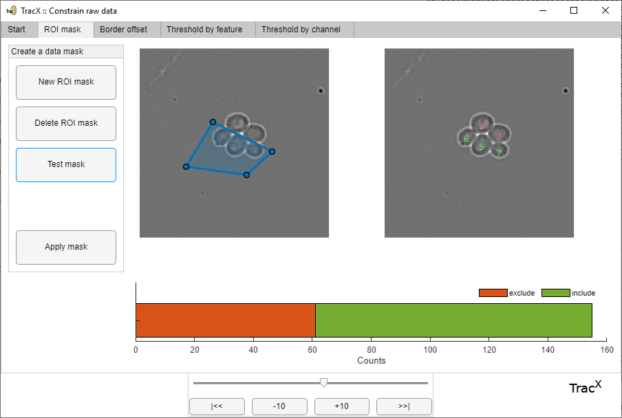
Constrain data¶

The constrain data window of Trac^x lets you constrain your (input) data prior to tracking. It is useful to remove segmentation artefacts or constrain tracking to a certain part of the image.

Constrain by a region of interest (ROI). This lets you select specific parts of the image to track.

Constrain by a image border offset. This lets you remove cells from the image borders which are often only partly segmented.

Constrain by segmentation feature. This lets you subset the data by any segmentation feature. I.e if you find that in your segmentation results you have a lot of small false positive segmentations you can set a threshold on cell_area such that only big segmentation objects will be considered.

Constrain by fluorescence. This lets you subset the data by any fluorescence channel. This is usefull to remove segmentation artefacts (dirt or other particles) since artefacts do not have an cellular background fluorescence and can be excluded this way.

Manual corrections¶

Manual track assignment correction tab¶

Trac^x does not require a manual ground truth to evaluate the track assignment correctness. With the fraction cell region fingerprint with values between 0 and 1 with 0 equal to no better assignment possible to 1 most likely there is a better one. However there are between 1-5% false positives especially if your imaging frequency was too low or you have a lot of changing neighbourhoods on the images. To deal with this you can change the Threshold (tau) to a higher number if you see that most of the potential errors are in fact correct assignments.

To correct assignment errors you can either process them by clicking the buttons By frac, By frame, By track. This will either sort the errors by fraction, by all tracks on a frame or by all tracks. In the table on the left you can then see the potential errors highlighted in orange and manually edit the track number by clicking into the field and change the number. On the right there are always three image frames displayed; The current one as well as the previous and following to help you identify if an assignment is correct or not and if not what it would need to be. With the slider and navigation buttons at the bottom you can move the current frame. Additionally you also see the tracking costs displayed. They help you understand where a potential error might be or if there are errors but not catch since the costs are too low this indicates that the Trac^x configuration was not optimal and it is worth the test a different set of parameters to avoid manual correction.

If you need to zoom into the images to better read a track number just hover over one and then a zoom icon will be displayed.

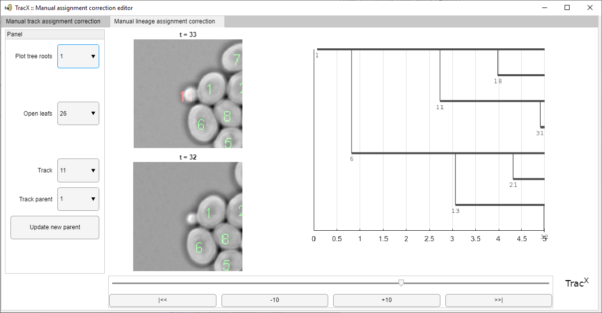
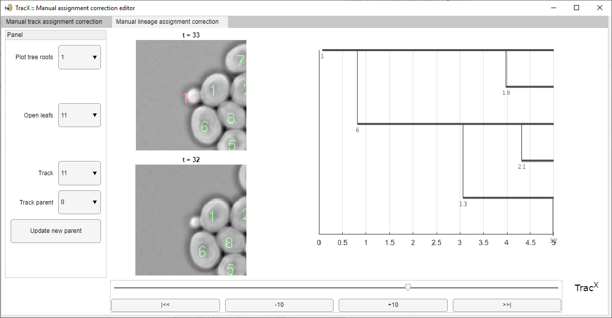
Manual lineage assignment correction tab¶

In case the automated lineage reconstruction did not result in what you were expecting you can annotate/fix parents manually. In the example below for asymmetric dividing yeast _S.cerevisiae_ cell 1 misses its daughter cell 11. In TracX the mother-daughter assignments are viewd from the daughter perspective. Therefore in this example cell 11 has parent 0 and is therefore a non-assigned leaf. To fix we select under open leaf or track cell 11 and then assign its parent 1 by selecting it from the drop down. The images highlight the current cell 11 (red label). To save the new assignment hit the Update new parent button.

Note

If the current time is not telling, you can select any other timepoint with the controls at the bottom and zoom or drag the images with the menu that shows up when placing the mouse over the image.

Tree before correction:

Tree after correction, showing cell 11 as daughter of cell 1.